这是一份很久以前一份作业报告.
第一题
加载工具包
输入要研究的股票数据代码
Show the code
#######################################
####输入要研究的股票数据代码#####
######################################
## 中国银行 601988.SS
##  中国建设银行 601939.SS
##  农行   601288.SS
## 浦发银行 600000.SS
## 民生银行  600016.SS
#下载数据
title<-"浦发银行" #股票名字作为图片标题 ,
stock<- "600000.SS"  # 股票的代码
sDate<-"2015-1-1" #开始日期
eDate<-"2018-10-01" #结束日期
下载数据并保存到本地
Show the code
## 上面的参数 eval=FALSE 代码这代码块不执行
download<-function(stock,from=sDate,to=eDate){
      df<-getSymbols(stock,from=from,to=to,env=environment(),auto.assign=FALSE)  #下载数据
      names(df)<-c("Open","High","Low","Close","Volume","Adjusted")
      write.zoo(df,file=paste(stock,".csv",sep=""),sep=",",quote=FALSE) #保存到本地
}


download(stock) # 这个是从网上下载数据,如果只研究一只股票,建议运行第一次以后,进行注释改代码
读取本地股票数据
Show the code
#本地读数据
read<-function(stock){
  as.xts(read.csv.zoo(file=paste(stock,".csv",sep=""),header = TRUE,sep=",", format="%Y-%m-%d"))
}


data <- read(stock)
cdata = data$Close
删除该文件
Show the code
file.remove(paste0(stock,".csv")) # 删除存储的文件计算日、月、年、收益率(按收盘价) 并保存数据
Show the code
daily_return=dailyReturn(cdata) # 日收益率
monthly_return = monthlyReturn(cdata) # 月收益率
yearly_return = yearlyReturn(cdata)  # 年收益率

# #保存股票的日收益率
# write.zoo(daily_return,paste0(stock,"_daily_return.csv"),
#           quote = FALSE, sep = ",")

# #保存股票的月收益率
# write.zoo(monthly_return,paste0(stock,"_monthly_return.csv"),
#           quote = FALSE, sep = ",")


# #保存股票的日收益率
# write.zoo(yearly_return,paste0(stock,"_yearly_return.csv"),
#           quote = FALSE, sep = ",")
计算 日收益率的均值 和波动率
计算移动平均值(5,10,20,60期移动平均值) 并保存数据
Show the code
#移动平均
ma<-function(cdata,mas=c(5,10,20,60)){
     ldata<-cdata
     for(m in mas){
         ldata<-merge(ldata,SMA(cdata,m))
     }
    #      ldata<-na.locf(ldata, fromLast=TRUE) #是否把NA进行均值填充
     names(ldata)<-c('Value',paste('ma',mas,sep=''))
     return(ldata)
 }

ldata = ma(cdata , c(5,10,20,30,60))  # 股票的 5 ,10 ,20 ,60 期移动平均值

# # 保存股票的 5 ,10 ,20 ,60 期移动平均值
# write.zoo(ldata,paste0(stock,"_",title,"_ma.csv"),quote = FALSE, sep = ",")
画出收盘价与5 期 30 期移动平均线
寻找金叉死叉,即买卖点
Show the code
ma_lag_data=function(ldata){
    SMA5 = embed (ldata[,2],2)  # 5期均线
    colnames(SMA5)= c("sam5","lagsma5")

    SMA30 = embed (ldata[,3],2) # 30期均线
    colnames(SMA30) = c("sma30","lagsma30")
    # 合并长期短期的sma
    smaLS=cbind(SMA5,SMA30)

    ## 转换为时间序列格式
    smaLS = xts(smaLS,order.by = index(ldata[,2][-1]))
    smaLS = na.omit(smaLS)
    return(smaLS)
}

smaLS = ma_lag_data(ldata)
保存买卖点
Show the code
## 构造捕捉向上突破点函数
Upcross<-function(x){
  ifelse(x[2]<x[4] & x[1]>x[3], 1, 0)
}

## 构造捕捉向下突破点函数
Downcross<-function(x){
  ifelse(x[2]>x[4] & x[1]<x[3], -1, 0)
}


# 捕捉短线 向上突破长线日期
Upsig<-apply(smaLS,1,Upcross)
Upsig<-xts(Upsig,order.by=index(smaLS))
names(Upsig)<-"Upsig"

# 捕捉短线 向上突破长线,释放买入信号,进行买入操作
UpBuy = lag.xts(Upsig) # 判断成功以后 要过后1期进行购买

## 查看所有买入点
UpBuy[UpBuy==1]
#>            Upsig
#> 2015-03-16     1
#> 2015-05-27     1
#> 2015-06-05     1
#> 2015-09-09     1
#> 2015-12-23     1
#> 2016-02-16     1
#> 2016-04-07     1
#> 2016-04-20     1
#> 2016-05-31     1
#> 2016-07-28     1
#> 2016-08-01     1
#> 2016-11-10     1
#> 2017-01-23     1
#> 2017-05-25     1
#> 2017-07-13     1
#> 2017-09-07     1
#> 2017-11-23     1
#> 2018-01-12     1
#> 2018-07-25     1

## 捕捉短线向下突破 长线日期

Downsig<-apply(smaLS,1,Downcross)
Downsig<-xts(Downsig,order.by=index(smaLS))
names(Downsig)<-"Downsig"

## 短线向上突破 长线,释放卖出信号,进行卖出操作
DownSell<-lag.xts(Downsig) # 判断成功以后 要过后1期进行购买
## 查看所有卖出点
DownSell[DownSell==-1]
#>            Downsig
#> 2015-05-11      -1
#> 2015-06-04      -1
#> 2015-06-24      -1
#> 2015-12-18      -1
#> 2015-12-31      -1
#> 2016-03-15      -1
#> 2016-04-08      -1
#> 2016-05-11      -1
#> 2016-06-27      -1
#> 2016-07-29      -1
#> 2016-10-18      -1
#> 2016-12-20      -1
#> 2017-03-02      -1
#> 2017-07-07      -1
#> 2017-08-09      -1
#> 2017-10-27      -1
#> 2017-12-15      -1
#> 2018-02-14      -1
dim(DownSell)
#> [1] 885   1
dim(UpBuy)
#> [1] 885   1


## 买卖数据点 1为买入,-1 为卖出  0 持有点
BSdata=DownSell+UpBuy
names(BSdata)="BS"

# 保存买卖数据点
# write.zoo(BSdata,paste0(stock,"_",title,"_买卖点.csv"),quote = FALSE, sep = ",")
在图上画出买卖点,并表示标签,买入(B),卖出(S),
Show the code
UpBuy1 = UpBuy[UpBuy==1]  # ## 查看所有买入点
DownSell1 = DownSell[DownSell==-1]## 查看所有卖出点

drow_plot_2ma = function(ldata,upbuytime,upbuylabel="B",downselltime,downselllabel="S",ptitle=title){
  ### ldata字段包含"Value"(收盘价) "ma5"(移动平均)   "ma20"
         plot1= dygraph(ldata,main = ptitle)%>%
           dyOptions(colors = c("red","blue", "green"),gridLineColor = "lightblue") %>%
            dyAxis("x", drawGrid = FALSE) %>%
              dyAxis("y", label = "price(价格)") %>%
                  dySeries(names(ldata)[2], strokeWidth = 2, strokePattern = "dashed") %>%
                        dySeries(names(ldata)[3], strokeWidth = 2, strokePattern = "dashed") %>%
                        dyRangeSelector()


           for(i in upbuytime){
             plot1 = plot1 %>%  dyAnnotation(i, text = upbuylabel, tooltip = "Korea")
           }

           for(j in downselltime){
             plot1 = plot1 %>%  dyAnnotation(j, text = downselllabel, tooltip = "Vietnam")
           }

  plot1
}


drow_plot_2ma(ldata = ldata,
              upbuytime = as.character(index(UpBuy1)),
              downselltime = as.character(index(DownSell1))
              )
画出所用的均线5,10,30,60 图 以及 收盘价 以及 2均线形成(5,30)的金叉死叉
Show the code
ldata = ma(cdata, c(5,10,30,60))

drow_plot_ma = function(ldata,upbuytime,upbuylabel="B",downselltime,downselllabel="S",ptitle=title){
  ### ldata字段包含"Value"(收盘价) "ma5"(移动平均)   "ma20"
         plot1= dygraph(ldata,main = ptitle)%>%
                    dyOptions(colors = RColorBrewer::brewer.pal( length(names(ldata)), "Set2")) %>%
                      dySeries(names(ldata)[1], strokeWidth = 2) %>%
                       dyAxis("x", drawGrid = FALSE) %>%
                         dyAxis("y", label = "price(价格)") %>%
                            dyRangeSelector()

         for( i in names(ldata)[2:length(names(ldata))]){
              plot1 = plot1 %>% dySeries(i, strokeWidth = 1, strokePattern = "dashed")
         }

           for(i in upbuytime){
             plot1 = plot1 %>%  dyAnnotation(i, text = upbuylabel, tooltip = "Korea")
           }

           for(j in downselltime){
             plot1 = plot1 %>%  dyAnnotation(j, text = downselllabel, tooltip = "Vietnam")
           }

  plot1
}


drow_plot_ma(ldata = ldata,upbuytime = as.character(index(UpBuy1)),downselltime = as.character(index(DownSell1)))
Show the code
library(ggplot2)
## 用ggplot2 画线图 首先对ldata数据进行整合
library(ggfortify)


## 快速画图


ldata = ma(cdata, c(5,30))


drow_ggplot2_ma=function(ldata,upbuytime,upbuylabel="B",downselltime,downselllabel="S",ptitle=title){
          plot2 = autoplot.zoo(ldata,facet = NULL) + labs(title=title, x="time", y="price")+theme(plot.title = element_text(hjust = 0.5))
           for(i in upbuytime){
             plot2 =plot2+ annotate("text", x=as.Date(i), y=as.numeric(ldata[i]$Value), label=upbuylabel)
           }

           for(j in downselltime){
             plot2=plot2+ annotate("text", x=as.Date(j), y=as.numeric(ldata[j]$Value), label=downselllabel)
           }
   plot2
}

drow_ggplot2_ma(ldata = ldata,upbuytime = as.character(index(UpBuy1)),downselltime = as.character(index(DownSell1)))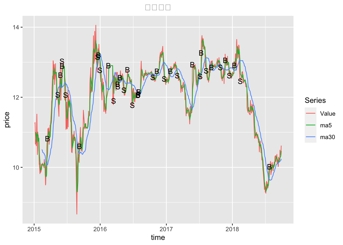
Show the code
ldata = ma(cdata, c(5,10,30,60))
drow_ggplot2_ma(ldata = ldata,upbuytime = as.character(index(UpBuy1)),downselltime = as.character(index(DownSell1)))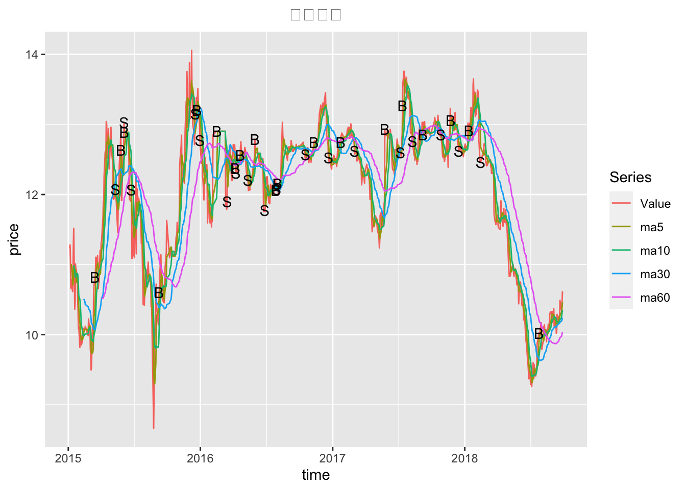
第二题 –VaR
输入要研究的股票数据代码
Show the code
#######################################
####输入要研究的股票数据代码#####
######################################
## 中国银行 601988.SS
##  中国建设银行 601939.SS
##  农行   601288.SS
## 浦发银行 600000.SS
## 民生银行  600016.SS
#下载数据
title<-"浦发银行" #图片标题
stock<-"600000.SS"  # 中国银行的代码
sDate<-"2015-1-1" #开始日期
eDate<-"2017-12-31" #结束日期
下载数据并保存到本地
Show the code
## 上面的参数 eval=FALSE 代码这代码块不执行
download<-function(stock,from=sDate,to=eDate){
      df<-getSymbols(stock,from=from,to=to,env=environment(),auto.assign=FALSE)  #下载数据
      names(df)<-c("Open","High","Low","Close","Volume","Adjusted")
      write.zoo(df,file=paste(stock,".csv",sep=""),sep=",",quote=FALSE) #保存到本地
}


download(stock) # 这个是从网上下载数据,如果只研究一只股票,建议运行第一次以后,进行注释改代码
读入数据
删除该文件
Show the code
file.remove(paste0(stock,".csv")) # 删除存储的文件计算VaR–历史模拟法
Show the code
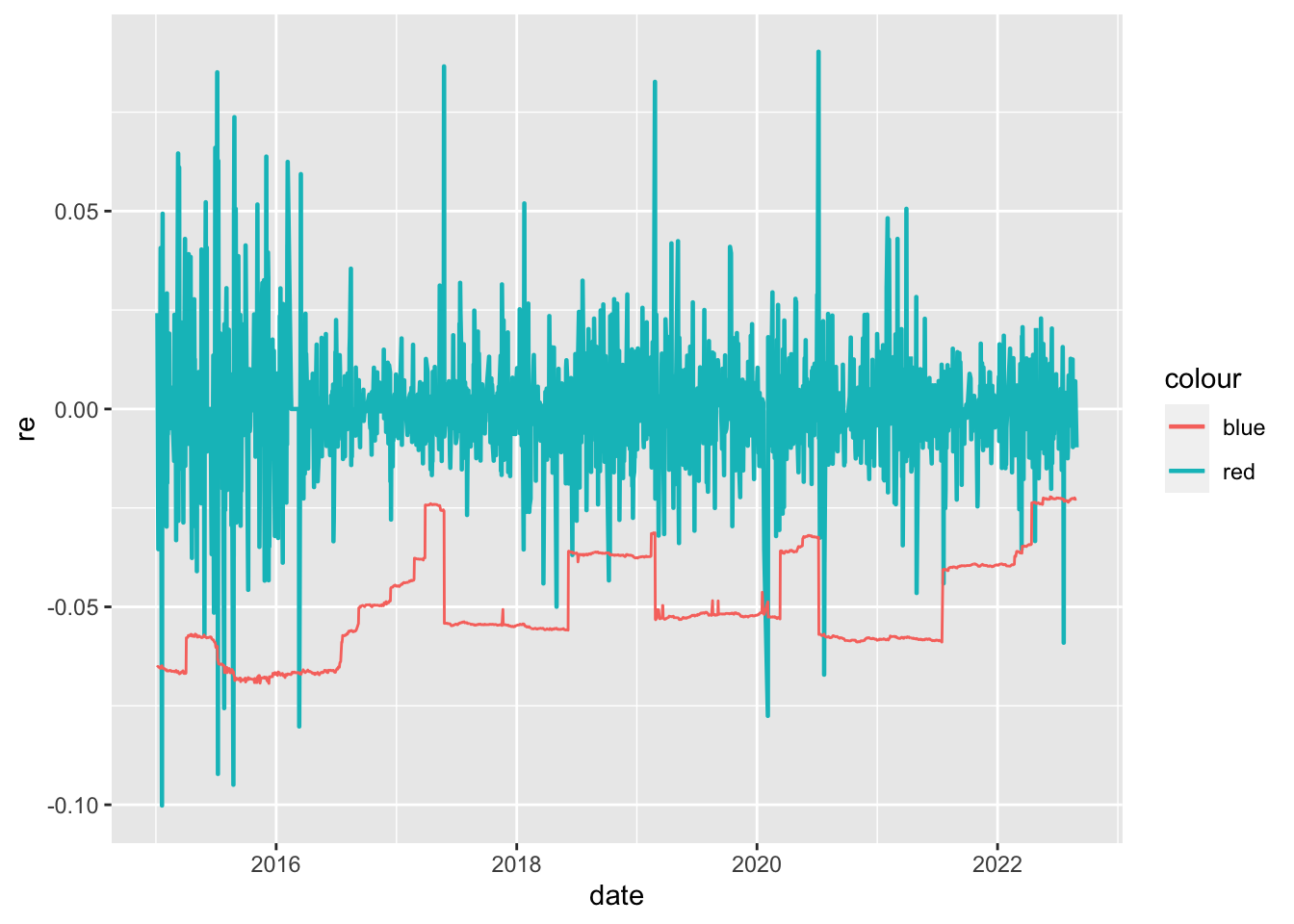
daily_return=dailyReturn(cdata)[-1] #cdata为收盘价,计算日收益率
daily_return_VaR =apply(embed(daily_return,90), 1, function(x)VaR(x,p=0.95,method = "historical")) %>% xts(.,order.by = index(daily_return[-c(1:89)]))

vardata = cbind(daily_return,daily_return_VaR)
names(vardata) =c("dreturn","d.re.var")
### 画出VaR时序图
dygraph(vardata,main = "日收益率与VaR") %>% dyRangeSelector() %>% dyAxis("y", label = "日收益率") %>% dyAxis("x", label = "时间")计算VaR–韦伯法
Show the code
library(quantmod)

ddd=xdata=getSymbols('600000.SS',auto.assign = F)
cdata<-data.frame(coredata(xdata))

names(cdata)<-c('open','high','low','close','volume','adjprice')
cdata$date<-as.Date(.indexDate(xdata))
n<-nrow(cdata)
cdata$re=NA
cdata$re[2:n]<-(cdata$close[2:n]-cdata$close[1:(n-1)])/cdata$close[1:(n-1)]## 计算日收益率

cdata=dplyr::filter(cdata,is.na(cdata$re)==F) #去除na值
n<-nrow(cdata) #提取

m<-sum(cdata$date>"2015-01-01") # 大于某个日期的天数

xdate<-cdata$date[cdata$date>"2015-01-01"] # 提前大于某个日期的天数
VaR<-rep(NA,m)
qVaR<-rep(NA,m)
zVaR<-rep(NA,m)
wVaR<-rep(NA,m)
d1=0
d2=0
d3=0
d4=0
alpha=0.05
for(i in 1:m){
  RE<-cdata$re[(n-m-252+i):(n-m+i-1)]
  SRE<-sort(RE)
  VaR[i]<--(SRE[trunc(252*alpha)]+SRE[trunc(252*alpha)+1])/2
  qVaR[i]<--quantile(RE,0.05)
  zVaR[i]<--qnorm(alpha,mean(RE),sd(RE))
  ERE<-exp(RE)
  fn<-function(par0){
    k<-par0[1]
    lambda<-par0[2]
    kk=0
    for(j in 1:252){
      x=ERE[j]
      kk=kk+
        log((k/lambda)*((x/lambda)^(k-1))*exp(-(x/lambda)^k))
    }
    return(kk)
  }
  xml <- optim(c(1,1),fn,method='BFGS',control=list(fnscale=-1))
  k   <- xml$par[1]
  lambda <- xml$par[2]
  wVaR[i] <- -log(qweibull(alpha,k,lambda))
  dre = cdata$re[n-m+i]

  if(dre < -VaR[i]){d1=d1+1}
  if(dre < -qVaR[i]){d2=d2+1}
  if(dre < -zVaR[i]){d3=d3+1}
  if(dre < -wVaR[i]){d4=d4+1}
}
ctv<-qbinom(0.05,m,alpha)
VR=data.frame(xdate,VaR,qVaR,zVaR,wVaR)
# plot(xdate,zVaR,type='l',col='blue')
# lines(xdate,VaR)

require(ggplot2)
VR1=data.frame(date=xdate,VAR=VaR,gr=rep('HIS',m))
VR2=data.frame(date=xdate,VAR=qVaR,gr=rep('qHIS',m))
VR3=data.frame(date=xdate,VAR=zVaR,gr=rep('Norm',m))
VR4=data.frame(date=xdate,VAR=wVaR,gr=rep('Weibull',m))

# xaa=rbind(VR1,VR2,VR3,VR4)
#
# ggplot(xaa,aes(x=date,y=VAR,group=gr,color=gr))+geom_line(size=0.8)
#
Show the code
Show the code
sessionInfo()
#> R version 4.2.1 (2022-06-23)
#> Platform: aarch64-apple-darwin20 (64-bit)
#> Running under: macOS Monterey 12.5.1
#>
#> Matrix products: default
#> BLAS:   /Library/Frameworks/R.framework/Versions/4.2-arm64/Resources/lib/libRblas.0.dylib
#> LAPACK: /Library/Frameworks/R.framework/Versions/4.2-arm64/Resources/lib/libRlapack.dylib
#>
#> locale:
#> [1] en_US.UTF-8/en_US.UTF-8/en_US.UTF-8/C/en_US.UTF-8/en_US.UTF-8
#>
#> attached base packages:
#> [1] stats     graphics  grDevices utils     datasets  methods   base
#>
#> other attached packages:
#>  [1] PerformanceAnalytics_2.0.4 ggfortify_0.4.14
#>  [3] RColorBrewer_1.1-3         dygraphs_1.1.1.6
#>  [5] lubridate_1.8.0            dplyr_1.0.9
#>  [7] stringr_1.4.1              scales_1.2.1
#>  [9] ggplot2_3.3.6              quantmod_0.4.20
#> [11] TTR_0.24.3                 xts_0.12.1
#> [13] zoo_1.8-10                 plyr_1.8.7
#>
#> loaded via a namespace (and not attached):
#>  [1] tidyselect_1.1.2  xfun_0.32         purrr_0.3.4       lattice_0.20-45
#>  [5] colorspace_2.0-3  vctrs_0.4.1       generics_0.1.3    htmltools_0.5.3
#>  [9] yaml_2.3.5        utf8_1.2.2        rlang_1.0.4       pillar_1.8.1
#> [13] glue_1.6.2        withr_2.5.0       DBI_1.1.3         lifecycle_1.0.1
#> [17] munsell_0.5.0     gtable_0.3.0      htmlwidgets_1.5.4 evaluate_0.16
#> [21] labeling_0.4.2    knitr_1.40        fastmap_1.1.0     curl_4.3.2
#> [25] fansi_1.0.3       Rcpp_1.0.9        jsonlite_1.8.0    farver_2.1.1
#> [29] gridExtra_2.3     digest_0.6.29     stringi_1.7.8     grid_4.2.1
#> [33] quadprog_1.5-8    cli_3.3.0         tools_4.2.1       magrittr_2.0.3
#> [37] tibble_3.1.8      crayon_1.5.1      tidyr_1.2.0       pkgconfig_2.0.3
#> [41] assertthat_0.2.1  rmarkdown_2.16.1  rstudioapi_0.14   R6_2.5.1
#> [45] compiler_4.2.1