--- title: GA包---遗传算法 date: '2015-11-09' categories: r --- ```{r setup, include=FALSE} :: opts_chunk$ set (echo = TRUE ,collapse = T, comment = "#> " )``` - 2022年3月23更新- 参考: [ Genetic Algorithms • GA (luca-scr.github.io) ](https://luca-scr.github.io/GA/) ## 1、用法:(默认求解最大值) - 注意: **默认求解最大值**```R ga (type = c ("binary" , "real-valued" , "permutation" ), # fitness:适应度函数 #解得下界/解得上界(多元变量为一个向量) #一个种群用二进制编码的长度是多少(长度越大代表精度越高,一般等于变量的个数即可) population = gaControl (type)$ population, # 初始种群 selection = gaControl (type)$ selection, #选择 crossover = gaControl (type)$ crossover, #交叉 mutation = gaControl (type)$ mutation, #变异 popSize = 50 , #种群大小 pcrossover = 0.8 , #交叉概率(默认0.8) pmutation = 0.1 , #变异概率(默认0.1) elitism = base:: max (1 , round (popSize* 0.05 )), #代沟(默认情况下,前5%个体将在每个迭代中保留) updatePop = FALSE ,postFitness = NULL ,maxiter = 100 , # 最大迭代次数(默认100) run = maxiter, #表示连续出现一定数目的目标函数值未改变,则GA终止搜索 maxFitness = Inf , # 适应度函数的上界,GA搜索后中断 names = NULL , # 表示决策变量名的向量 suggestions = NULL , # 包含某些指定的初始种群 optim = FALSE , # optim默认值为FALSE,用于确定是否应使用使用通用优化算法的局部搜索。有关更多详细信息和更精细的控制,请参阅参数optimArgs。 # 简单理解, 即optim= T时, 表面进过一定次数的迭代后从 GA 最优解开始最为 optim函数的初始值,开始进行局部优化 # optimArgs 控制本地搜索算法的列表,具有以下组件: optimArgs = list (method = "L-BFGS-B" , # 可以是optim函数中的方法 poptim = 0.1 ,# 范围[0,1]中的值,指定在每次GA迭代时执行局部搜索的概率(默认值为0.1)。 pressel = 0.5 ,control = list (fnscale = - 1 , maxit = 100 )),keepBest = FALSE , #一个逻辑参数,指定每次迭代的最佳解决方案是否应该保存在一个名为 bestSol 的槽中。 parallel = FALSE , #是否采用并行运算 monitor = if (interactive ()) #绘图用的,监控遗传算法的运行状况 if (is.RStudio ()) gaMonitor else gaMonitor2 } else FALSE ,seed = NULL ) #一个整数值包含随机数发生器的状态。这个参数可以用来复制GA搜索的结果。 ``` ## 2、参数说明 ``` type: 解得编码类型 1. binary :二进制编码 2. real-valued:实数浮点编码 3. permutation:问题涉及到重新排序的列表,字符串编码。可求解TSP问题 通过gaControl设置默认的遗传算子。检索当前设置操作: gaControl(“binary”) gaControl(“real-valued”) gaControl(“permutation”) ``` ## 3.举例 ### 3.1. 一元函数: - 函数为: $ |x|+cos(x) $- 该函数有最小值$ f(0)=1(−R \leq x \leq R)$```{r} rm (list = ls ())library (GA)= function (x) abs (x)+ cos (x)curve (f, - 20 , 20 )``` ```{r} = function (x) - f (x) #由于这个函数默认求解最大值,所以我们求-f(x)的最大值 = ga (type = "real-valued" , fitness = fitness, lower = - 20 , upper = 20 ,monitor= F)# monitor 禁止打印信息 ##返回的结果GA为S4对象,一个GA类型 调用其属性用@符号 @ solution # 返回最优解 summary (GA)## 画图--- 展示迭代信息 plot (GA) # #默认情况下,ga函数通过打印每个迭代的平均值和最佳适应度值来监视搜索,画出每代最佳的适应度函数值与每代的平均适应度函数值 # ####画出最优值 # curve(f, -20, 20) # # abline(v = GA@solution, lty = 3) ``` ```{r} ### binary 测试 = ga (type = "binary" , fitness = fitness, nBits = 1 ,lower = - 20 , upper = 20 ,monitor= F)@ solution # 返回最优解 ``` ```{r} :: pkg_load2 ('gifski' ) # 安装并加载该软件包 ######################## ##编写自己的跟踪功能,点代表一个解,来监视搜索 ## 定义一个新的监视器函数,然后将此函数作为可选参数传递给ga: = function (obj) { curve (f, - 10 , 10 , main = paste ("iteration =" , obj@ iter))points (obj@ population, obj@ fitness, pch = 20 , col = 2 )rug (obj@ population, col = 2 )Sys.sleep (0.2 )}## 监视函数-- 运行了会输出很多静态图 # GA = ga(type = "real-valued", fitness = f, lower = -10, upper = 10, monitor = monitor) ```  ```{r} ############## ## 也可以储存为视频,观看,利用动画的函数做出视频 # library(animation) # oopts = ani.options(ffmpeg = "F:/ffmpeg/bin/ffmpeg.exe")#在winds中设置ffmpeg # saveVideo({ # #打印图片 # GA = ga(type = "real-valued", fitness = f, lower = -10, upper = 10, monitor = monitor) # ani.options(interval = 0.1, nmax = 250) # }, video.name = "jianshi.mp4", other.opts = "-b 500k") # ################ ``` ### 3.2. 二元函数: ```{r} rm (list = ls ())= function (x1, x2) {20 + x1^ 2 + x2^ 2 - 10 * (cos (2 * pi * x1) + cos (2 * pi * x2))# 画图 # x1 = seq(-5.12, 5.12, by = 0.1) # x2 = seq(-5.12, 5.12, by = 0.1) # f = outer(x1, x2, Rastrigin) # persp3D(x1, x2, f, theta = 50, phi = 20)# 3D图 # filled.contour(x1, x2, f, color.palette = jet.colors)# 热力图 = function (obj) {contour (x1, x2, f, drawlabels = FALSE , col = gray (0.5 ))title (paste ("iteration =" , obj@ iter), font.main = 1 )points (obj@ population, pch = 20 , col = 2 )Sys.sleep (0.2 )= ga (type = "real-valued" , fitness = function (x) - Rastrigin (x[1 ], x[2 ]),lower = c (- 5.12 ,- 5.12 ), upper = c (5.12 , 5.12 ), popSize = 50 , maxiter = 100 , monitor = NULL ) #定义monitor,暂时不运行 @ solution``` ### 3.3 最小二乘法 ### 3.4 子集的选择 `UsingR` 包中加载数据集,然后通过OLS拟合线性回归模型:```{r} rm (list = ls ()):: pkg_load2 ("UsingR" )data ("fat" , package = "UsingR" )#252*19 = lm (body.fat.siri ~ age + weight + height + + chest + abdomen + + thigh + knee + ankle + + forearm + wrist, data = fat)#通过观察,因变量(body.fat.siri) 与上述 13个自变量有关系 summary (mod)``` ```{r} = model.matrix (mod)[, - 1 ] # 252*13 选取13 个自变量的列,构建自变量 = model.response (model.frame (mod)) # 提取因变量的列, ###### 那么,最大化的适应度函数可以定义为: = function (string) {= which (string == 1 )= cbind (1 , x[,inc])= lm.fit (X, y)class (mod) = "lm" - AIC (mod)``` ```{r} = ga ("binary" , fitness = fitness, nBits = ncol (x),names = colnames (x),monitor = F,parallel = T)# monitor = plot @ solution#####利用GA找到的最优子集得到的线性回归模型如下: = lm (body.fat.siri ~ .,data = data.frame (body.fat.siri = y, x[,GA@ solution == 1 ]))summary (mod2)``` ### 3.5 约束优化 - 约束优化,可以通过对目标函数加入惩罚函数来实现,即不在约束范围内的目标函数值设置为 $- \infty$`利润(p),权重(w)和容量(V):` ```{r} rm (list = ls ())= c (6 , 5 , 8 , 9 , 6 , 7 , 3 )= c (2 , 3 , 6 , 7 , 5 , 9 , 4 )= 14 ##### 利用二进制遗传算法可以解决背包问题,但由于不等式约束,并不是所有可行解都可行。 ##### 我们可以通过惩罚不可行的解决办法来考虑约束。因此,适应度函数可以定义如下: = function (x) {= sum (x * p)= sum (w) * abs (sum (x * w)- V)- penalty##### 当目标函数f被惩罚时,一个量取决于提出的解决方案的容量与背包容量之间的距离。然后: = ga (type = "binary" , fitness = knapsack, nBits = length (w),maxiter = 1000 , run = 200 , popSize = 20 )@ solution# 解 sum (p * GA@ solution)sum (w * GA@ solution)``` ### 3.7. 解决TSP问题  ```R 1 ,2 ]表示城市A与城市B之间的距离,于是D[1 ,2 ]= 7,同时也表示我现在处于A–1城市,将要去B–2城市; ``` ```{r,eval=F } rm (list = ls ())#city数据结构 一共有31个城市,计算出每两个城市之间的距离,用距离矩阵表示 = as.matrix (dist (city)) # 距离矩阵 #定义总的路线长度 = function (tour, distMatrix) {= c (tour, tour[1 ]) #设置为回路,代表所走的路径 = embed (tour, 2 )[,2 : 1 ]#根据回路,产生对应的距离矩阵的下标,每一行代表一个坐标,第一行处于i坐标 sum (distMatrix[route])= function (tour, ...) 1 / tourLength (tour, ...)= ga (type = "permutation" , fitness = tspFitness, distMatrix = D,lower = 1 , upper = dim (D)[1 ], popSize = 50 , maxiter = 5000 ,run = 500 , pmutation = 0.2 ,monitor = F, parallel = T)summary (GA3)apply (GA3@ solution, 1 , tourLength, D)#找到的解决方案对应于一条独特的路径,其行程长度等于: ``` ```{r,eval=F} library (ggplot2)library (tibble)= rownames_to_column (city, var = "rowname" )#原始图像 # p=ggplot(data=city,aes(x=X1,y=X2))+geom_point(shape=19,size=4,col="red")+theme_bw()+ # geom_text(aes(label=rowname),size=4,vjust=1.5)+geom_path(linetype=2)+ggtitle("初始顺序") library (dplyr)= data.frame (solution= as.factor (GA3@ solution[1 ,]))= inner_join (city_solution,city,by= c ("solution" = "rowname" ))#re_city #最优解城市顺序 ##最优解城市图像 = ggplot (data= re_city,aes (x= X1,y= X2))+ geom_point (shape= 19 ,size= 4 ,col= "red" )+ theme_bw ()+ geom_text (aes (label= solution),size= 4 ,vjust= 1.5 )+ geom_path (linetype= 2 )+ ggtitle ("最优解" )+ geom_point (x= re_city[1 ,2 ],y= re_city[1 ,3 ],shape= 17 ,size= 5 ,col= "blue" )+ theme (plot.title = element_text (hjust = 0.5 )) + theme (text= element_text (family= "Songti SC" ))``` 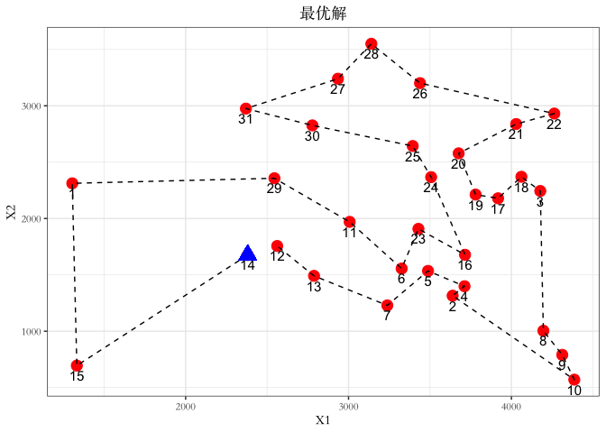 ```{r} sessionInfo ()```