matlab优化工具04二次规划之quadprog
二次规划问题是目标函数为 \(\textbf{x}\) 的二次形式, 约束条件为线性等式或不等式约束
二次规划的一般模型
\[ \begin{aligned} \min \quad & f^T x + \frac{1}{2}x^T \textbf{H} x \\ \text {s.t.} \quad & \textbf{A} \cdot x \leq b \\ & \textbf{Aeq} \cdot x=beq \\ & l b \leq x \leq ub \end{aligned} \]
其中: \(x, b, beq\)是向量, \(f^T\) 为一次项的系数, \(\textbf{A}\)是矩阵,\(\textbf{H}\)是矩阵, \(\textbf{H}\)是矩阵,即二次项系数,用以描述\(x_i^2\) 以及 \(x_i x_j\)项. \(\textbf{A}\)线性不等式,\(\textbf{Aeq}\)线性等式,
当然,二次规划的目标函数中的二次项还可以用元素的形式表达,即 \[ \begin{aligned} \frac{1}{2}\left(h_{11} x_{1}^{2}+h_{12} x_{1} x_{2}+\cdots+h_{1 n} x_{1} x_{n}+h_{21} x_{1} x_{2}+h_{22} x_{2}^{2}+\cdots+h_{n n} x_{n}^{2}\right) \end{aligned} \]
定理: 如果\(\textbf{H}\) 矩阵为正定矩阵, 则二次规划问题是凸问题. 即它的求解与初始值无关,只要有可行解,则一定是全局最优解.
如果二次规划问题非凸,则该函数不能得出原始问题的全局最优解,甚至可能不能得出可行解.
matlab 函数— — quadprog
%% 语法
x = quadprog(H,f,A,b,Aeq,beq,lb,ub)
x = quadprog(H,f,A,b,Aeq,beq,lb,ub,x0)
x = quadprog(H,f,A,b,Aeq,beq,lb,ub,x0,options)
x = quadprog(problem)
[x,fval,exitflag,output,lambda] = quadprog(___)

%% 不解释了, 看前面的fmincon函数
x0 初始值
例1
\[ \begin{aligned} min & \quad \left(x_{1}-1\right)^{2}+\left(x_{2}-2\right)^{2}+\left(x_{3}-3\right)^{2}+\left(x_{4}-4\right)^{2} \\ & \text{s.t.} \begin{cases} x_{1}+x_{2}+x_{3}+x_{4} \leqslant 5 \\ 3 x_{1}+3 x_{2}+2 x_{3}+x_{4} \leqslant 10 \\ x_{1}, x_{2}, x_{3}, x_{4} \geqslant 0 \end{cases} \end{aligned} \]
方法一: 根据上述方程,写出标准形式的二次规划
\[ f(x)=x_{1}^{2}+x_{2}^{2}+x_{3}^{2}+x_{4}^{2}-2 x_{1}-4 x_{2}-6 x_{3}-8 x_{4}+30 \]
然后写出 \(\textbf{H}\)和\(f^T\),代码如下:
clc,clear all;format compact;
f = [-2;-4;-6;-8];
H = diag([2,2,2,2]);
A = [1,1,1,1;
    3,3,2,1];
b = [5;10];
lb = [0,0,0,0];
ub = [];
x0=[];
options = optimoptions('quadprog','Display','iter');
[x,fval,exitflag,output,lambda] = quadprog(H,f,A,b,[],[],lb,ub,x0,options)
% ---------------------------- 结果 -------------------------
x =
    0.0000
    0.6667
    1.6667
    2.6667
fval =
  -23.6667
方法2 : 采用问题描述的形式 — 结构体
这种模式,不需要手工推导\(\textbf{H}\) 矩阵
%% 问题描述形式 --- 以结构体方式创建
%%
% optimproblem('ObjectiveSense','max')  % 最优化问题的创建,  ObjectiveSense属性求最大值(默认最小值)
%%  optimvar 决策变量的定义,n,m,k 设置决策变量的维度,不设置k则变量维度为n*m
% x = optimvar('x',n,m,k,'LowerBound',lb,'UpperBound',ub)


clc,clear all;format compact;
x = optimvar('x',4,1,'LowerBound',[0;0;0;0],'UpperBound',[]);
objec = sum( (x - [1;2;3;4]).^2 );
prob = optimproblem('Objective',objec);
prob.Constraints.cons1 = sum(x) <= 5;
prob.Constraints.cons2 = 3*x(1) + 3*x(2) + 2*x(3) + x(4) <=10;
sols = solve(prob);
x=sols.x

%% ---------------------------- 结果 -------------------------
x =
    0.0000
    0.6667
    1.6667
    2.6667

%% 上述问题还可以简化,利用向量的形式给出
clc,clear all;format compact;
x = optimvar('x',4,1,'LowerBound',[0;0;0;0],'UpperBound',[]);
objec = sum( (x - [1:4]').^2 );
prob = optimproblem('Objective',objec);
prob.Constraints.cons1 = sum(x) <= 5;
prob.Constraints.cons2 = [3,3,2,1] * x <=10;
sols = solve(prob);
x=sols.x

%% ---------------------------- 结果 -------------------------
x =
    0.0000
    0.6667
    1.6667
    2.6667
例2:
\[ \begin{aligned} \min \quad & -2 x_{1}+3 x_{2}-4 x_{3}+4 x_{1}^{2}+2 x_{2}^{2}+7 x_{3}^{2}-2 x_{1} x_{2}-2 x_{1} x_{3}+3 x_{2} x_{3} \\ & \text{s.t. }\begin{cases} 2 x_{1}+x_{2}+3 x_{3} \geq 8 \\ x_{1}+2 x_{2}+x_{3} \leq 7 \\ -3 x_{1}+2 x_{2} \leq-5 \\ x_{1}, x_{2}, x_{3} \geq 0 \end{cases} \end{aligned} \]
由于上述问题采用手工的方法比较麻烦,因此可以采用问题描述的形式求解该问题
clc,clear all;format compact;
x = optimvar('x',3,1,'LowerBound',[0;0;0],'UpperBound',[]);
objec = -2*x(1) + 3*x(2) - 4*x(3) + 4*x(1)^2 + 2*x(2)^2 + 7*x(3)^2 -2*x(1)*x(2) -2*x(1)*x(2) + 3*x(2)*x(3);
prob = optimproblem('Objective',objec);
prob.Constraints.cons1 = [2,1,3] * x >= 8;
prob.Constraints.cons2 = [1,2,1] * x <=7;
prob.Constraints.cons3 = [-3,2,0] * x <= -5;
sols = solve(prob);
x=sols.x

%% ---------------------------- 结果 -------------------------
Solving problem using quadprog.
Your Hessian is not symmetric. Resetting H=(H+H')/2.

Minimum found that satisfies the constraints.

Optimization completed because the objective function is non-decreasing in
feasible directions, to within the value of the optimality tolerance,
and constraints are satisfied to within the value of the constraint tolerance.

<stopping criteria details>
x =
    2.2500
    0.8750
    0.8750
上述可以看到 Your Hessian is not symmetric. Resetting H=(H+H')/2. 说明给出了警告,指出自动生成的Hesse 矩阵是非对称的, 所以建议设置H=(H+H')/2 将其转化为对称矩阵. 由于问题描述模式没有输入H矩阵. 因此,应该将问题描述模式转为结构体模型,再来处理H矩阵(这样做不会产生警告,不过最后的结果都是一样的).
>> p = prob2struct(prob);
p =
  包含以下字段的 struct:

     intcon: []
         lb: [3×1 double]
         ub: [3×1 double]
         x0: []
      Aineq: [3×3 double]
      bineq: [3×1 double]
        Aeq: []
        beq: []
         f0: 0
     solver: 'quadprog'
          H: [3×3 double]
          f: [3×1 double]
    options: []
>> p.H = (p.H + p.H') / 2;
>> x1 = quadprog(p)
x1 =
    2.2500
    0.8750
    0.8750
双下标二次规划
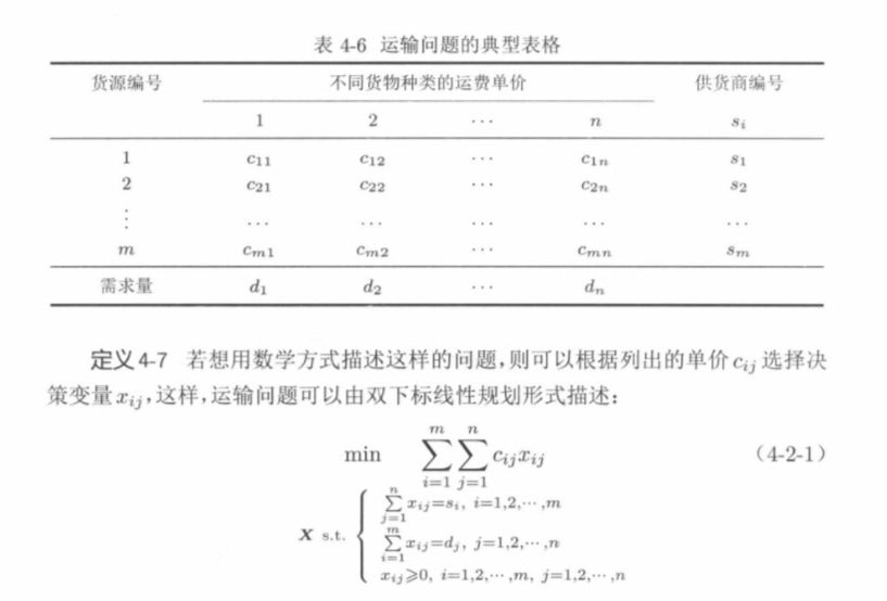
主要是根据线性模型中的运输问题直接扩展而来的, 即把线性模型中的运输问题的目标函数用二次项表示,其他的约束条件都不变
线性模型中的运输问题
双下标二次规划的一个改进版本 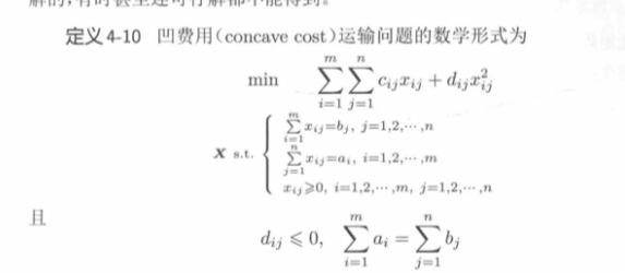
%%  对凹费用运输问题的求解,假设 n = 4, m = 6, a,b,C,D 已知;
%% 双虾标的运输问题(凹费用运输问题)
% 已知 n, m,a,b,C,D
clc,clear all;format compact;
n = 4; m = 6;
a = [8,24,20,24,16,12]';
b = [29,41,13,21];
C= [300, 270, 460, 800;
    740, 600, 540, 380;
    300, 490, 380, 760;
    430, 250, 390, 600;
    210, 830, 470, 680;
    360, 290, 400 ,310];
D = [-7, -4, -6, -8;
    -12, -9, -14, -7;
    -13, -12, -8, -4;
    -7, -9, -16, -8;
    -4, -10, -21, -13;
    -17,-9,-8,-4];

x = optimvar('x',m,n,'LowerBound',0,'UpperBound',[]);
objec = sum(sum(C .* x + D.* (x.^2)) );
prob = optimproblem('Objective',objec);
prob.Constraints.cons1 = sum(x,1) == b;
prob.Constraints.cons2 = sum(x,2) == a;
sols = solve(prob);
x=sols.x

%% ---------------------------- 结果 -------------------------
Solving problem using quadprog.
The problem is non-convex.
x =
     1     1     1     1
     1     1     1     1
     1     1     1     1
     1     1     1     1
     1     1     1     1
     1     1     1     1
>>
注意: 上述结果不满足约束条件,即得出的结果不是可行解, 这时候, 则需要使用fmincon 函数了
% 由于上述问题采用问题描述方式书写的,这里进行转化,转化为结构体模式
p = prob2struct(prob);
p.solver = 'fmincon'; %转为结构体必须修改必要的参数
f = @(x) sum(C(:) .* x + D(:) .* x.^2);
p.Objective = f; %定义目标函数
ff  = optimset;
ff.TolX =eps; % 一个比较苛刻的误差值l
ff.TolFun=eps;
p.options = ff;
p.x0 =100*rand(m*n,1);
x0 =fmincon_global(p,-10,10,n*m,50);
X0 = reshape(x0,m,n)

%% ---------------------------- 结果 -------------------------
X0 =
    6.0000    2.0000    0.0000    0.0000
    0.0000    3.0000    0.0000   21.0000
   20.0000    0.0000    0.0000    0.0000
    0.0000   24.0000    0.0000    0.0000
    3.0000    0.0000   13.0000    0.0000
    0.0000   12.0000    0.0000    0.0000
参考:
matlab函数官网
<<薛定宇教授大讲堂卷5 MATLAB最优化计算>>_含目录py.pdf