据我了解, 计算机软件中画的函数图像大概有两种方法:
- 方法一: 该图像有一系列密集点组成, 已达到欺骗人们的眼睛.感觉认为是连续的.
- 方法二: 为了解决方法一种的问题,把每两个点之间用直线连接已达到连续的状态
在本文中我们将利用R语言来画函数图像—- 重点以ggplot2来展示
1. \(y = f(x)\) 的函数图像
比如:
\[ \begin{aligned} y &= sin(x),\\ y &= cos(x), \\ y &= \dfrac{1}{1+e^{(-x)}},\\ y &= x^2 . \end{aligned} \]
这是我们中学最常见的函数.
方法一: curve()画函数图像
所用函数调用格式
curve(expr, from = NULL, to = NULL, n = 101, add = FALSE,
      type = "l", xname = "x", xlab = xname, ylab = NULL,
      log = NULL, xlim = NULL, ...)
# expr:函数名称或一个关于变量x的函数表达式;
# from,to:表示绘图的起止范围;
# n:一个整数值,表示x取值的数量;
# add:是一个逻辑值,当为TRUE时,表示将绘图添加到已存在的绘图中;
# type:与plot函数中type含义相同
#定义公式
sigmoid <- function(x) 1/(1+exp(-x))
#画sigmid图像
curve(sigmoid,-10,10)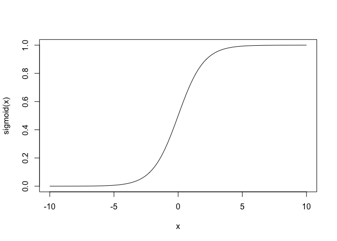
#画sin(x)函数图像
curve(sin,-10,10)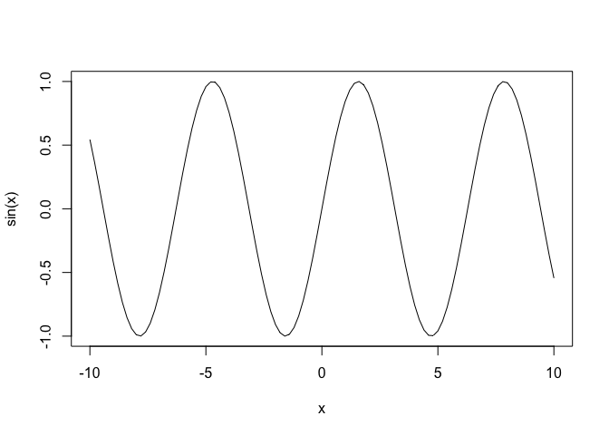
# 画y=x^2的图像
curve(x^2,-10,10)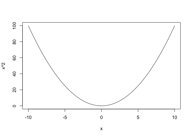
方法二: ggplot2
首先介绍两个映射
geom_path()按照观测值在数据中出现的顺序连接观测值(如果画函数图,推荐此映射,原因后面知晓)。geom_line()按变量在x轴上的顺序连接它们。
library(ggplot2)

# 定义函数
sigmoid <- function(x) 1/(1+exp(-x))

# 创建数据点
x<-seq(-5, 5, by=0.01)
y<-sigmoid(x)
df<-data.frame(x, y)

# 用ggplot2来画图
g <- ggplot(df, aes(x,y))
g <- g + geom_path(col='red') ## 用geom_line 替代也是可以的,但不推荐
g <- g + geom_hline(yintercept = 0.5) + geom_vline(xintercept = 0) #坐标轴
g <- g +  labs(title="sigmoid", x="x", y="y")
g <- g +theme(plot.title = element_text(hjust = 0.5))  #标题居中
g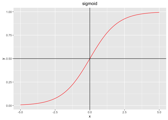
2. 函数图像具有参数方程
例如: 圆, 椭圆, 抛物线, 双曲线 方程.
2.1 画\(x^2+y^2 = 4\)的函数图像
这里我们只以ggplot2为例,
思路一: 可以利用分段函数的思想画,先把原函数解出显示的表达式 \(y = -\sqrt{4-x}\) 或者\(y = \sqrt{4-x}\), 然后分段画, 这里不讲解
思路二: 像上面这些函数,都能表示成参数方程的形式, 利用参数方程来画该函数图像
首先写出圆的参数方程一般形式:
\[ \begin{cases} x = rcos\theta,\\ y = rsin\theta \end{cases} \]
library(ggplot2)
r = 2
theta=seq(0, 2*pi, by=0.001)
x = r*cos(theta)
y = r*sin(theta)
df <- data.frame(x, y, theta,frame = 1:length(theta))
g <- ggplot(df, aes(x,y))
g <- g + geom_path(col='red')
g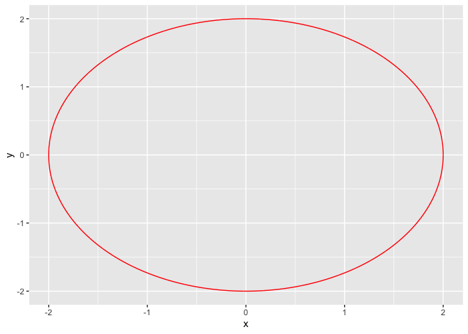
###################
####让上面的图动起来
library(gganimate)
library(transformr)
temp = g + transition_reveal(along = frame)

animate(temp,
        nframes=100,#总帧数(默认)
        duration=10 #总时长,单位为秒,默认为10秒
        )
2.2 椭圆
椭圆的参数方程
\[ \begin{cases} x = acos\theta,\\ y = bsin\theta \end{cases} \]
library(ggplot2)
a = 2
b = 3
theta=seq(0, 2*pi, by=0.001)
x = a*cos(theta)
y = b*sin(theta)
df <- data.frame(x, y, theta,frame = 1:length(theta))
g <- ggplot(df, aes(x,y))
g <- g + geom_path(col='red')
## 让图动起来
temp = g + transition_reveal(along = frame)

animate(temp)
2.3 抛物线
抛物线参数方程
\[ \begin{cases} x = 2pt^2, \\ y = 2pt \end{cases} (t为参数, t \in R) \]
p = 4
t = seq(3,-3,-0.2)
x = 2*p*t^2
y = 2*p*t
df <- data.frame(x, y, t,frame = 1:length(t))
g <- ggplot(df, aes(x,y))
g <- g + geom_path(col='red')
## 让图动起来
temp = g + transition_reveal(along = frame)

animate(temp)
2.4 双曲线
在ggplot中没有找到好的画法
a = 3
b = 1
theta=round(seq(0,2*pi,0.2),2)

x = a/cos(theta)
y = b*tan(theta)
df <- data.frame(x, y, theta,frame = 1:length(theta))
g <- ggplot(df, aes(x,y))
g <- g + geom_path(col='red')
g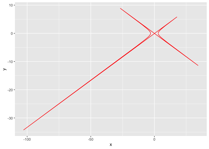
# 以分段的思想来画双曲线


x <- seq(1,3,length = 100)
y1 <- sqrt(x^2 - 1);y2 <- -sqrt(x^2 - 1)

xx1 = c(rev(x),x); yy1 = c(rev(y2),y1)

xx2 = c(rev(-x),-x);yy2 = c(rev(y2),y1)

df <- data.frame(xx1,yy1,xx2,yy2, frame = 1:length(xx1))
g <- ggplot(df) + geom_path(aes(xx1,yy1),col='red')
g <- g + geom_path(aes(xx2,yy2),col='blue')
g 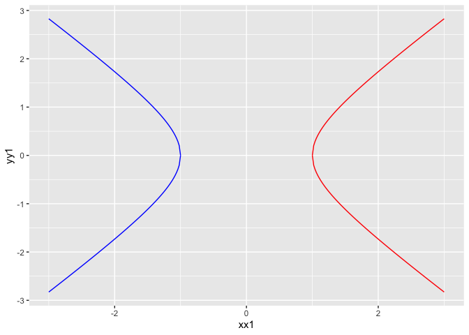
temp = g + transition_reveal(along = frame)

animate(temp)
2.4 Lissajous 曲线(利萨如曲线)
参数方程:
\[ \begin{cases} x = asin(p\theta),\\ y = 2sin(q\theta+\varphi) \end{cases} \]
a = 1
b = 1
phi = 0
p = 1
q = 2
t = seq(0, 2 * pi, by = 0.001)
x = a * sin(p * t)
y = b * sin(q * t + phi)
df <- data.frame(x, y, t, frame = 1:length(x))
g <- ggplot(df, aes(x, y))
g <- g + geom_path(col = 'red')

temp = g + transition_reveal(along = frame)

animate(temp)
a = 3
b = 12
phi = 0
p = 13
q = 18
t = seq(0, 2 * pi, by = 0.001)
x = a * sin(p * t)
y = b * sin(q * t + phi)
df <- data.frame(x, y, t, frame = 1:length(t))
g <- ggplot(df, aes(x, y))
g <- g + geom_path(col = 'red')
g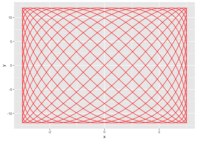
temp = g + transition_reveal(along = frame)

animate(temp)
3 .隐函数
这个暂时不知道, 且不常见,建议找MATLAB这种专业软件画或者ggb也行.